Differentials in housing costs and their impact on Malaysia's income inequality measures - Articles

Inequality measures are generally based on money incomes—household income, income per capita (per household member) or income per adult equivalent. Studies of income inequality often assume that households and individuals living in different parts of a country face the same set of prices, so differences in money income will fairly reflect differences in the purchasing power of income received—‘real income’.

Spatial variations in prices are to be expected in large economies like the United States (US) and China. Jolliffe (2006) found that allowing for cost-of-living differences between metropolitan and non-metropolitan areas in the US causes a complete reversal of the poverty ranking of these areas. He attributed spatial variation in the cost of living entirely to housing costs. Li and Gibson (2014) analysed the impact of spatial housing price variations on gross domestic product (GDP) inequality across regions of China, and found that ‘one-quarter of GDP inequality across regions disappears once account is taken of cost-of-living differences’ (p. 92).

Of course, Malaysia is far smaller than the US and China, both geographically and in population size. But variations in prices across Malaysia’s states have been of some public concern, and they are of much relevance for policy formulation. Data obtained from the Department of Statistics-Malaysia (DoS) confirm that the price of housing—an important item of spending—is far higher in urban areas, and especially in Malaysia’s capital, Kuala Lumpur (KL). Allowing for the effects of the price of housing on real income significantly lowers Malaysia’s income inequality metrics in both 2009 and 2016, with the improvement strengthening somewhat in 2016. Based on money income, the relative poverty rate in KL was 2.8 per cent in 2016, but when incomes are adjusted to reflect differential housing costs, the rate more than doubled to 6.6 per cent. And the proportion of rich individuals living in KL fell from a third to a fifth following the housing-cost adjustment.

In Putrajaya, housing costs now exceed those in Kuala Lumpur
Credit: iStock.com/Lina Moiseienko

Spatial variation in prices

Variations in the prices of traded goods can be expected to be relatively minor in Malaysia as competitive forces will act to equalise these prices—the ‘law of one price’. However, for non-traded goods and services like housing, prices can vary significantly across Malaysia’s states and strata (urban versus rural). DoS has provided the price data by state and stratum that are used in the construction of the Consumer Price Index (CPI) for 2009 and 2016. The CPI data reveal significant variations in the cost of housing (including utilities) across states and strata.

Indeed, it is becoming increasingly costly to live in KL (Figure 1). In 2009 and 2016, the cost of housing in KL was around 1.7 times the (unweighted) average cost of housing in other Malaysian urban areas. Compared with average housing costs in rural areas, KL housing was even costlier—1.9 and 2.8 times as expensive in 2009 and 2016, respectively.

These price differentials may partly reflect differences in housing quality. The price of housing in each state and stratum is a weighted average of housing sub-categories, like rent on single-storey detached property, rent on a low-cost flat, etc. As these weights vary by state and stratum, it is possible that the housing price variations may be due in part to variations in the housing-quality mix. This may well be the reason for the high price of housing in Putrajaya, the only state in 2016 where the housing cost exceeded that in KL. Nevertheless, the data confirm the widely held view that housing costs in the capital are well out of line with those in other parts of the country.

Figure 1 Housing costs elsewhere are generally lower than those in Kuala Lumpur

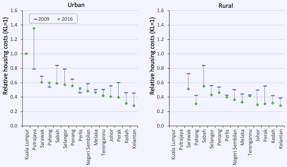
To enjoy a real standard of living comparable with elsewhere, individuals living in KL will need far more money income. Measures of inequality based simply on money income are likely to give a misleading impression of the distribution of real living standards.

To make comparisons of income reflect real living standards, household incomes require adjustment to take account of variations in the cost of housing. On the assumption that households purchase items other than housing at the same set of prices, we define adjusted—or real—income for each household as:

where Y is the household’s money income, w_h is the DoS CPI national budget weight (see https://bit.ly/2DrqFCU) for housing (23.8 per cent), and r_h is the price of housing in the household’s state and stratum relative to that faced by households in KL. Since the cost of housing carries a weight of around a quarter in the calculation of the CPI, housing price variations can be expected to have a major impact on our measure of real income. Of course the implicit assumption that the housing budget share does not vary across states and strata is unlikely to hold. Without further information on these budget shares, in what follows the constant CPI budget share for housing is applied to each household.

Spatial variations in the cost of housing make a difference to measures of real income inequality
Credit: iStock.com/taikrixel

Real and money incomes will be the same for households living in KL, since for these households r_h will equal one. For households living in states and strata where the costs of housing are below those in KL (r_h<1), real incomes will be above their corresponding money incomes. Intuitively, real income is the income that the household would need to reach its current standard of living if it were located in KL.

An example will illustrate the point. Consider an individual living in urban Johor earning an income of RM16,000 a year in 2016. The cost of housing there was just over 40 per cent of the housing cost in KL, r_h=0.4032. If this individual were living in KL, to enjoy the same standard of living she or he would need to earn:

To enjoy in KL the same standard of living currently enjoyed in urban Johor, she or he would need an income 35 per cent higher (21,636 over 16,000). This adjustment is typical across states in 2016, where the mean adjustment to money income was around 30 per cent (albeit somewhat lower in 2009 at 17 per cent).

Inequality in real and money incomes

How do inequality measures based on real incomes differ from those based on unadjusted money incomes? Income is defined as total gross household income from the 2009 and 2016 Household Income Surveys, divided by the number of adult equivalents in the household. This ‘equivalised income’ concept is widely used in the analysis of income distribution. (Similar results were obtained when analysing household income per capita, so these are not reported here.) Income comprises paid employment income, other earned income, property income and transfers. The number of adult equivalents is based on the modified OECD¹ scheme: 1 for the first adult in the household, 0.5 for the second and each additional member aged 14 and over, and 0.3 for each child under 14.

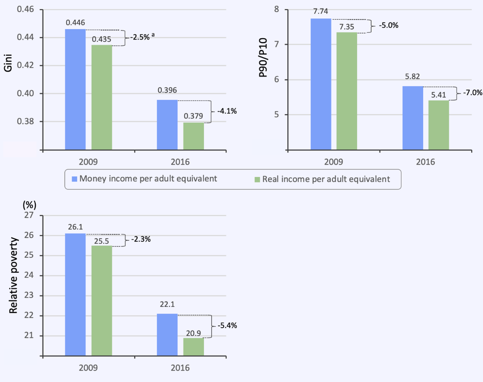
Figure 2 shows three measures of inequality for Malaysia: the Gini coefficient, the P90/P10 ratio (the ratio of the income of the poorest individual in the top decile to that of the richest individual in the poorest decile) and the relative poverty rate (the proportion of individuals receiving less than 60 per cent of the median). The three indices are measured over individuals rather than households.

Inequality measures based on real incomes were all lower than those based on money income, and the effect on inequality was somewhat stronger in 2016 than in 2009. In 2016, the Gini based on real income was 4.1 per cent lower than that based on money income (0.379 against 0.396), and the P90/P10 was 7 per cent lower (5.41 versus 5.82). Through the application of ‘jackknife’ standard errors, the Gini coefficients based on real income in 2009 and 2016 were all significantly lower than those based on money income. The incidence of relative poverty in 2016 was 5.4 per cent lower with adjusted incomes. Real incomes were therefore more equitably distributed than money incomes in both years.

Figure 2 Malaysia’s inequality measures based on real incomes are lower than those based on money incomes

^a Percentage differences.

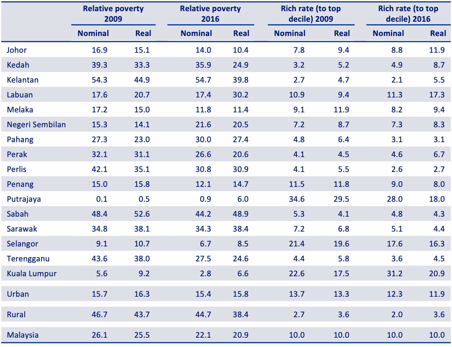
Where do the rich and poor live

Taking into account the observed costs of housing inevitably changes the spatial distribution of low and high incomes (Table 1). Rich individuals are defined as persons with equivalised income in Malaysia’s top decile. The most striking features are:

The 2016 relative poverty rate in KL more than doubles from 2.8 per cent when based on money income to 6.6 per cent for adjusted or real income.
In Putrajaya, the relative poverty rate in 2016 based on money income was less than 1 per cent, rising to 6 per cent when income is adjusted. This is hardly surprising as in 2016 the cost of housing in Putrajaya exceeded that in KL by 35 per cent (Figure 1, left panel).
The reverse effect is evident in Kedah and Kelantan, where relative poverty rates based on real income were substantially lower. Housing costs in these states were less than a third of those in KL.
In 2016, close to a third of people living in KL were in the top 10 per cent in money income terms. But when account is taken of the higher cost of housing in KL, only one fifth were in the top decile. Similarly, far fewer rich persons live in Putrajaya based on adjusted income.

TABLE 1 Where Malaysia’s relatively poor and rich live (%)

Conclusions

Allowing for spatial variations in the cost of housing makes a significant difference to measures of income inequality and, more dramatically, the locations of rich and poor individuals. With such variations, Malaysian inequality measures were lower in 2009 and 2016 than without them. In 2016, the Gini coefficient was 0.396 based on money income and 0.379 based on real income—a reduction of 4 per cent. The relative poverty rate of KL more than doubled in 2016 to 6.6 per cent when income is adjusted to reflect local housing costs. In 2016, close to a third of persons living in KL and Putrajaya were in the top decile of money income earners, a share that falls to a fifth for both areas when account is taken of their higher costs of housing. The results suggest the need for care in interpreting spatial differentials in income measures when variations in cost of living are not taken into account.

Especially in urban areas, housing occupies a large part of an individual’s or household’s expenditure. Regular publication of an index that accurately measures spatial differential in critical components of the cost of living could assist employers in determining cost-of-living allowances. The results also suggest the need to build affordable housing for low-income groups living in urban areas.

Data sources:

Both Household Income Surveys and the 2016 housing-price data used in this article were provided courtesy of the Economic History of Malaya project. The 2009 housing-price data were provided by DoS as part of the EPU-UNDP work on Malaysian poverty: Demery (2013), Table 5.

Note: ¹Organisation for Economic Co-operation and Development.

The fraction of Indians in Malaya’s population rose very sharply in the decades between 1901–1921, from just 6 per cent to 15 per cent, as rubber planting expanded and inflows were at their peak. But the Indian share of the population fell after 1931 and was just 11 per cent by 1947, as many Indian plantation workers were repatriated as a result of the rise in unemployment over the Great Depression years (Figure 1).

Beyond the plantations, Indians were recruited, inter alia, for public works, as police and guards, and also to serve in the lower ranks of the colonial bureaucracy. Most came from Tamil areas in south India. They were considered to be more accustomed to British rule, more amenable to discipline than the Chinese, and more willing to work for low wages. Access to low cost Indian labour migration helped ensure the rubber industry’s spectacular growth and profitability. Since there was work for wives and older children on the rubber estates, Indian migration included whole families. But low wages, indebtedness, poor social status, and physical isolation kept estate Indians apart and they tended to exercise little influence on Malayan society.

The fraction of Indians in Malaya’s population rose very sharply in the decades between 1901–1921, from just 6 per cent to 15 per cent, as rubber planting expanded and inflows were at their peak. But the Indian share of the population fell after 1931 and was just 11 per cent by 1947, as many Indian plantation workers were repatriated as a result of the rise in unemployment over the Great Depression years (Figure 1).

Beyond the plantations, Indians were recruited, inter alia, for public works, as police and guards, and also to serve in the lower ranks of the colonial bureaucracy. Most came from Tamil areas in south India. They were considered to be more accustomed to British rule, more amenable to discipline than the Chinese, and more willing to work for low wages. Access to low cost Indian labour migration helped ensure the rubber industry’s spectacular growth and profitability. Since there was work for wives and older children on the rubber estates, Indian migration included whole families. But low wages, indebtedness, poor social status, and physical isolation kept estate Indians apart and they tended to exercise little influence on Malayan society.

The fraction of Indians in Malaya’s population rose very sharply in the decades between 1901–1921, from just 6 per cent to 15 per cent, as rubber planting expanded and inflows were at their peak. But the Indian share of the population fell after 1931 and was just 11 per cent by 1947, as many Indian plantation workers were repatriated as a result of the rise in unemployment over the Great Depression years (Figure 1).

Beyond the plantations, Indians were recruited, inter alia, for public works, as police and guards, and also to serve in the lower ranks of the colonial bureaucracy. Most came from Tamil areas in south India. They were considered to be more accustomed to British rule, more amenable to discipline than the Chinese, and more willing to work for low wages. Access to low cost Indian labour migration helped ensure the rubber industry’s spectacular growth and profitability. Since there was work for wives and older children on the rubber estates, Indian migration included whole families. But low wages, indebtedness, poor social status, and physical isolation kept estate Indians apart and they tended to exercise little influence on Malayan society.

References:

Demery, David. 2013. ‘Revision of Malaysia’s Poverty Line Income’, report by the United Nations Development Programme (UNDP) for the Economic Planning Unit (EPU), Kuala Lumpur.

Jolliffe, Dean. 2006. ‘Poverty, prices, and place: How sensitive is the spatial distribution of poverty to cost-of-living adjustments?’, Economic Inquiry, 44(2), 296–310.

Li, Chao and John Gibson. 2014. ‘Spatial price differences and inequality in the People’s Republic of China: Housing market evidence’, Asian Development Review, 31(1), 92–120.